
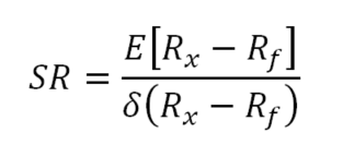
Financial academics as well as practitioners for long have come up with “risk-adjusted” metrics to be able to evaluate the quality of investments, strategies and funds and to compare them apple to apple. The most common metric used is Sharpe Ratio introduced by American economist William Sharpe in 1966 who won Nobel prize in Economics in 1990 for developing “Capital Asset Pricing Model“. He defined ex-ante Sharpe Ratio as the ratio of the expected excess return of the asset over risk-free rate and its standard deviation as a risk metric.
There are other similar risk-adjusted return metrics that use different measures of risk in the denominator such as Sortino Ratio (using standard deviation of negative returns) and Treynor Ratio (using Beta of the strategy as risk measure). Ex-post version of these measures are used to evaluate the performance of the fund in the realized past. Wider (and much late) acceptance of the findings by Benoit Mandelbrot in 1963 that in financial returns, volatility tends to cluster (i.e. absolute or square of returns show strong auto-correlation) has finally helped the realization that Sharpe Ratio could be a little misleading risk-adjusted return metric and it doesn’t fully reflect the reward and pain investors go through an investment. Mandelbrot showed that volatility clusters (correlated absolute returns), returns were not following a Gaussian (normal) distribution and hence standard deviation of them could be meaningless.
Even if you wrongly assume the returns follow a normal distribution, consider the following, the two 1-year equity curves below have the same ex-post Sharpe Ratio of around 1. (for both CAGR=~20%, VOL=~20%)

Yet just by looking at these two curves and their drawdowns, we know that investors have two totally different experiences which cannot be expressed by a risk-adjusted return metric of Sharpe Ratio=1.
So in summary, Sharpe Ratio has following drawbacks:
- Returns are not normally distributed and hence standard deviation could be meaningless
- Volatility clustering is not reflected in it
- It doesn’t reflect the real pain investors experience
- Two investments with equal Sharpe Ratios could have completely dissimilar paths in terms of reward and risk
- it is boundless (as the ratio of two independent variables, theoretically it is not limited)
It was shown later on that drawdowns (especially deeper drawdowns when panic ensues in the markets) follow more of a Power Law distribution. So a better metric for risk and the pain investors go through emerged: Maximum Drawdown. It is the maximum percentage of fall that investors experience from the previous high that investment has reached. It is this fall from the highs that inflicts pain on investors and limits the leverage investors could take in any investment without being ruined not the standard deviation of returns. In other words, a maximum drawdown of 100% is blow up and the absorbing barrier. No investment survives after such drawdown.
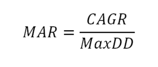
If we define risk as MaxDD, then a suitable risk adjusted metric could be a combination of return and MaxDD. MAR ratio introduced in 1978 by Leon Rose is one such risk-adjusted return metric. It was introduced in the Managed Accounts Report newsletter and gets its name from that publication. It is the ratio of Compound Annual Growth Rate (CAGR) and Maximum Drawdown (MaxDD):
By using MaxDD as risk measure, it is an improvement on Sharpe Ratio, however it has its own problems in adjusting the return. MAR ratio punishes shallow drawdowns more than deeper ones for example, for two strategies with equal return but with MaxDD1=10% and MaxDD2=20%, MAR drops in half for the second strategy. However imagine two other strategies with equal return and following MaxDDs: MaxDD1=80% and MaxDD2=90%. For these two MAR1 is only 1.125 times the MAR2. Both these strategies are horrible in terms of the risk imposing on the investors but the second strategy is much much more riskier than the first one because as the drawdowns get deeper, it gets exponentially tougher to recover from them. A strategy in 80% drawdown needs 5x return to get back to previous high while a strategy in 90% drawdown requires a 10x return to get back to previous high! a 2x difference. This goes to show the strong force of compound returns works equally strongly in the negative side and good investments should avoid compounding negative returns. Traders on wall street jokingly emphasize this point: “Do you know what is a 90% drawdown? it is when you’re down 80% and then your money is cut in half!”
So we need a better metric to accurately reflect the reality of negative compounding and punish deeper drawdowns more not the reverse. Based on this discussions so far, I propose a new risk-adjusted return metric called Effective Return (ER). Here is the definition of ER:
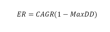
I define the effective return as multiplication of Compound Annual Growth Rate (CAGR) by (1-MaxDD). MaxDD is defined as percentage and is always below 1, so 1-MaxDD is always a positive number below 1 and as a result ER is always a number lower than CAGR.
By defining Effective Return in this way, return is adjusted for the pain investors experience to recover from the maximum drawdown throughout the fund growth and ups and downs. If a fund experiences 80% maximum drawdown, which as we said needs a 5x return to get back to previous high, it means ER equals CAGR * (1-0.8) = CAGR * 0.2, and if a fund goes through a drawdown of 90%, its ER will be CAGR * (1-0.9) = CAGR * 0.1 which will be half of previous fund’s ER. Notice here we reduce CAGR by MaxDD to get ER and so it makes sense to call this new metric Effective Return.
Because ER is bounded by CAGR, it cannot go to infinity even if we have a very low volatility fund. It is limited by the CAGR of the fund.
So in summary, Effective Return (ER):
- Doesn’t assume normality of returns
- Considers the clustering of volatility (maximum drawdown instead of standard deviation)
- Accurately reflects the pain investors feel through drawdowns by multiplying a haircut to the return (CAGR)
- It correctly punishes deeper drawdowns much more than shallow drawdowns
- It is bounded by the return (CAGR)
- Has the drawback of depending on MaxDD which depends on the duration of fund or strategy or its inception time
For example, for S&P500 total return daily index (SPXTR) from 1/1/1990 to 10/29/2021:

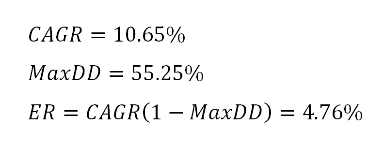
By proposing ER as a new risk-adjusted return metric, I hope to bring much more attention to the need for controlling drawdowns in investment strategies and appropriately encourage strategies that provide returns at much lower drawdowns for investors.
Leave a Reply